Which nonlinear dimension reduction methods preserve outliers inside a sphere?

Last updated on Aug 30, 2020 3 min read

In this post we will look at how well nonlinear dimension reduction techniques preserve outliers that are placed inside a sphere, when all the other data points are on the surface of the sphere. We will use the R package dimRed for this analysis. First we note that linear projection-based methods on the original data will not work, because projections will hide the outliers inside the sphere. Also, none of the nonlinear dimension reduction methods we consider are especially designed for outlier detection. So, it is not a limitation of the method if they do not preserve outliers. But, we want to see if any of them do.

Let’s plot the data first.

set.seed(1)
theta <- seq(from = -1*pi, to = pi, by=0.01)
phi <- seq(from = 0, to= pi*2, by=0.01)
theta1 <- sample(theta, size=5*length(theta), replace=TRUE)
phi1 <- sample(phi, size=5*length(phi), replace=TRUE)
x <- cos(theta1)*cos(phi1)
y <- cos(theta1)*sin(phi1)
z <- sin(theta1)

df <- cbind.data.frame(x,y,z)
df1 <- df
dim(df)

## [1] 3145    3

oo <- matrix(c(0,0,0,0,0.2,-0.1), nrow=2, byrow = TRUE)
colnames(oo) <- colnames(df)
df <- rbind.data.frame(df, oo)
plot(df[ ,c(1,2)], pch=20)
points(df[3146:3147, ], pch=20, col=c("red", "green"), cex=2)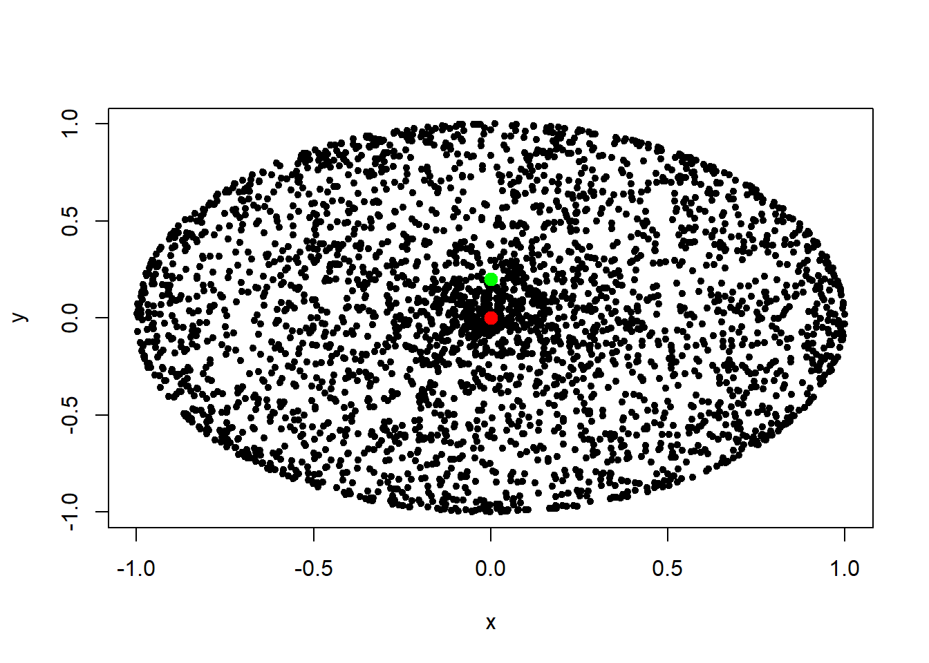

dd2 <- dimRedData(df)

The dataframe contains 3145 points on the surface of the sphere. These points are non-outliers. The data points in the dataframe on rows 3146 and 3147 are the outliers. We plot the outliers in red and green.

Most methods need a parameter such as \(k\) in KNN distances. For all methods we fix \(k=10\) and map the original data from \(\mathbb{R}^3\) to \(\mathbb{R}^2\). It is also called a 2-dimensional embedding. Let’s start our analysis with IsoMap.

IsoMap

emb2 <- embed(dd2, "Isomap", .mute = NULL, knn = 10)

## 2020-08-30 23:17:23: Isomap START

## 2020-08-30 23:17:23: constructing knn graph

## 2020-08-30 23:17:23: calculating geodesic distances

## 2020-08-30 23:17:27: Classical Scaling

embdat <- as.data.frame(emb2@data)
plot(embdat, pch=20,main="IsoMap embedding")
points(embdat[3146:3147, ],  pch=20, col=c("red", "green"), cex=2)

Well, \(k=10\), did not bring out the outliers inside the sphere using IsoMap. Next, let’s look at Locally Linear Embedding (LLE).

LLE

emb2 <- embed(dd2, "LLE", knn = 10)

## finding neighbours
## calculating weights
## computing coordinates

embdat <- as.data.frame(emb2@data)
plot(embdat, pch=20, main="LLE embedding")
points(embdat[3146:3147, ], pch=20, col=c("red", "green"), cex=2)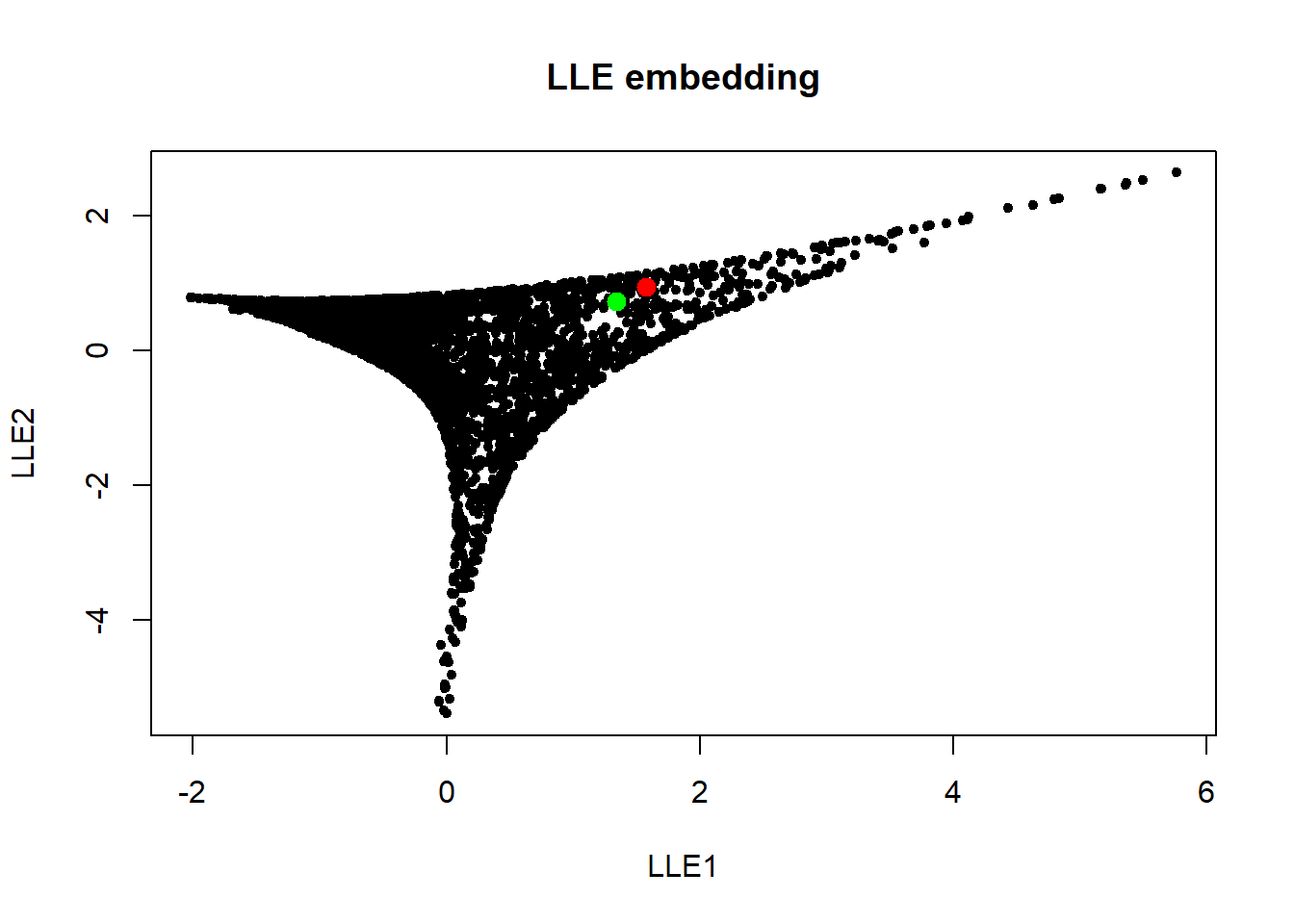

Next we look at Laplacian Eigenmaps.

Laplacian Eigenmaps

emb2 <- embed(dd2, "LaplacianEigenmaps", knn = 10)

## 2020-08-30 23:00:51: Creating weight matrix

## 2020-08-30 23:00:52: Eigenvalue decomposition

## Eigenvalues: 5.098969e-03 3.829450e-03 4.537894e-17

## 2020-08-30 23:00:53: DONE

embdat <- as.data.frame(emb2@data)
plot(embdat, pch=20, main="Lapacian eigenmaps embedding")
points(embdat[3146:3147, ], pch=20, col=c("red", "green"), cex=2)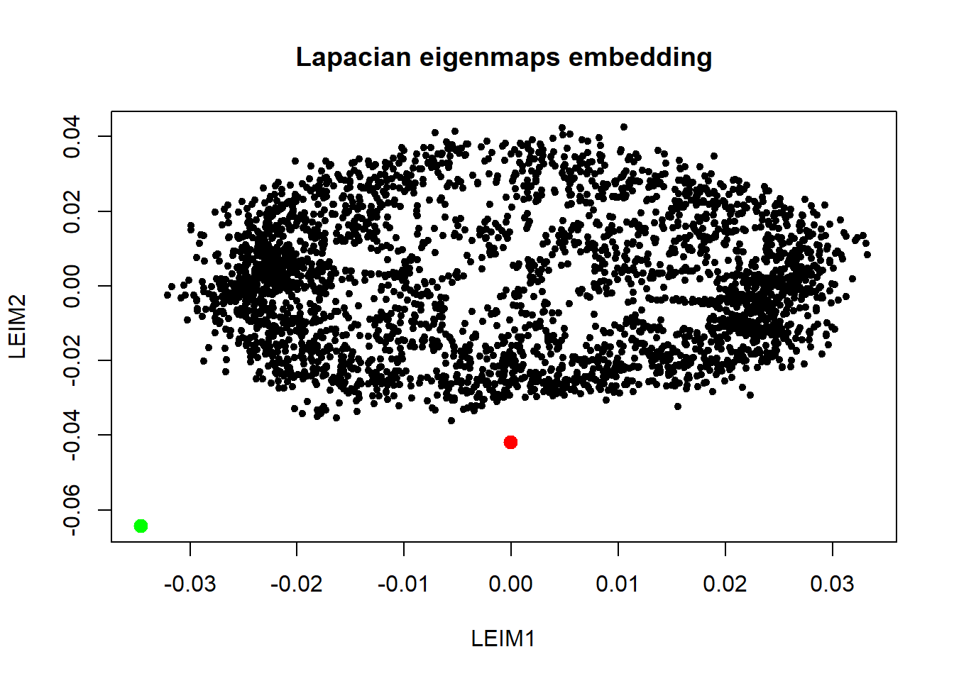

This is nice. Laplacian eigenmaps really brought out the outliers using \(k=10\). Next we look at diffusion maps.

Diffusion Maps

emb2 <- embed(dd2, "DiffusionMaps")

## Performing eigendecomposition
## Computing Diffusion Coordinates
## Elapsed time: 4.67 seconds

embdat <- as.data.frame(emb2@data)
plot(embdat, pch=20, main="Diffusion maps embedding")
points(embdat[3146:3147, ],  pch=20, col=c("red", "green"), cex=2)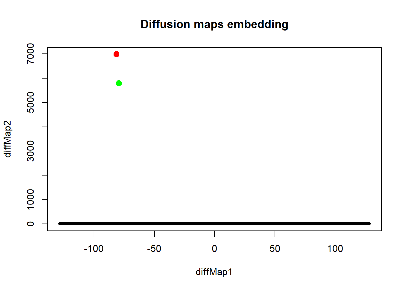

Diffusion maps also brought out the outliers. Interestingly, everything else is mapped to a line. Next we consider non-metric dimensional scaling.

Non-Metric Dimensional Scaling

emb2 <- embed(dd2, "nMDS", d = function(x) exp(dist(x)))

embdat <- as.data.frame(emb2@data)
plot(embdat, pch=20, main="non-MDS embedding")
points(embdat[3146:3147, ], pch=20, col=c("red", "green"), cex=2)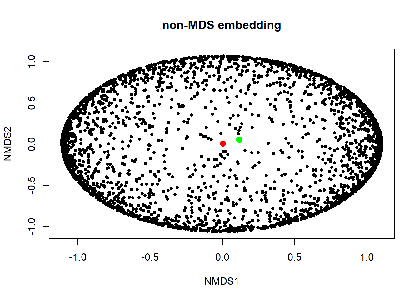

Finally we do tsne.

tsne

emb2 <- embed(dd2, "tSNE", perplexity = 10)

embdat <- as.data.frame(emb2@data)
plot(embdat, pch=20, main="tsne embedding")
points(embdat[3146:3147, ], pch=20, col=c("red", "green"), cex=2)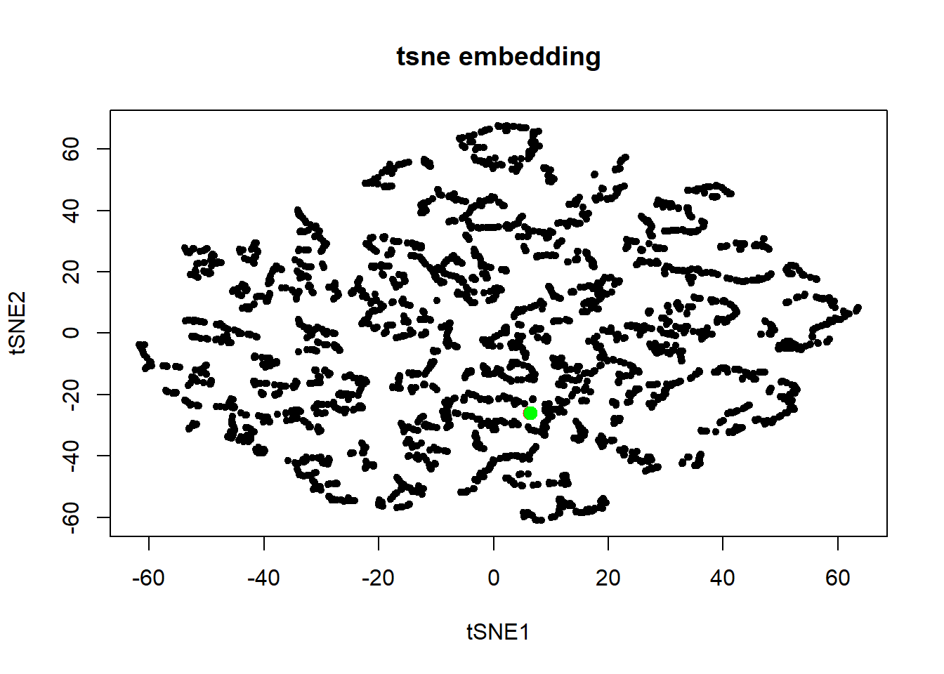

Of the methods explored, Laplacian eigenmaps brought out the outliers while showing some spherical structure in the embedding. Diffusion maps also brought out the outliers. However, the spherical structure of the data was lost in the embedding.